Overview

BigQuery is Google's fully managed, NoOps, low cost analytics database. With BigQuery you can query terabytes and terabytes of data without having any infrastructure to manage or needing a database administrator. BigQuery uses SQL and can take advantage of the pay-as-you-go model. BigQuery allows you to focus on analyzing data to find meaningful insights.

This lab focuses on how to architect a data warehouse for query performance. In this lab, you will compare a traditional relational schema with joins against a denormalized schema. You will also use BigQuery's Query Execution Plan to quantifiably assess performance trade-offs.

What you'll do

In this lab, you will learn how to perform these tasks:

• Load a comma-separated value (CSV) file into a BigQuery table using the web UI.
• Load a JavaScript® Object Notation (JSON) file into a BigQuery table using the command-line interface (CLI).
• Transform data and join tables using the web UI.
• Store query results in a destination table.
• Query a destination table using the web UI to confirm your data was transformed and loaded correctly.

Setup and requirements

For each lab, you get a new Google Cloud project and set of resources for a fixed time at no cost.

1. Sign in to Qwiklabs using an incognito window.

2. Note the lab's access time (for example, 1:15:00), and make sure you can finish within that time.
   There is no pause feature. You can restart if needed, but you have to start at the beginning.

3. When ready, click Start lab.

4. Note your lab credentials (Username and Password). You will use them to sign in to the Google Cloud Console.

5. Click Open Google Console.

6. Click Use another account and copy/paste credentials for this lab into the prompts.
   If you use other credentials, you'll receive errors or incur charges.

7. Accept the terms and skip the recovery resource page.

Activate Google Cloud Shell

Google Cloud Shell is a virtual machine that is loaded with development tools. It offers a persistent 5GB home directory and runs on the Google Cloud.

Google Cloud Shell provides command-line access to your Google Cloud resources.

1. In Cloud console, on the top right toolbar, click the Open Cloud Shell button.

   

2. Click Continue.

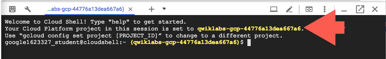
It takes a few moments to provision and connect to the environment. When you are connected, you are already authenticated, and the project is set to your PROJECT_ID. For example:

gcloud is the command-line tool for Google Cloud. It comes pre-installed on Cloud Shell and supports tab-completion.

• You can list the active account name with this command:

Output:

Example output:

• You can list the project ID with this command:

Output:

Example output:

Open BigQuery Console

1. In the Google Cloud Console, select Navigation menu > BigQuery.

The Welcome to BigQuery in the Cloud Console message box opens. This message box provides a link to the quickstart guide and lists UI updates.

2. Click Done.

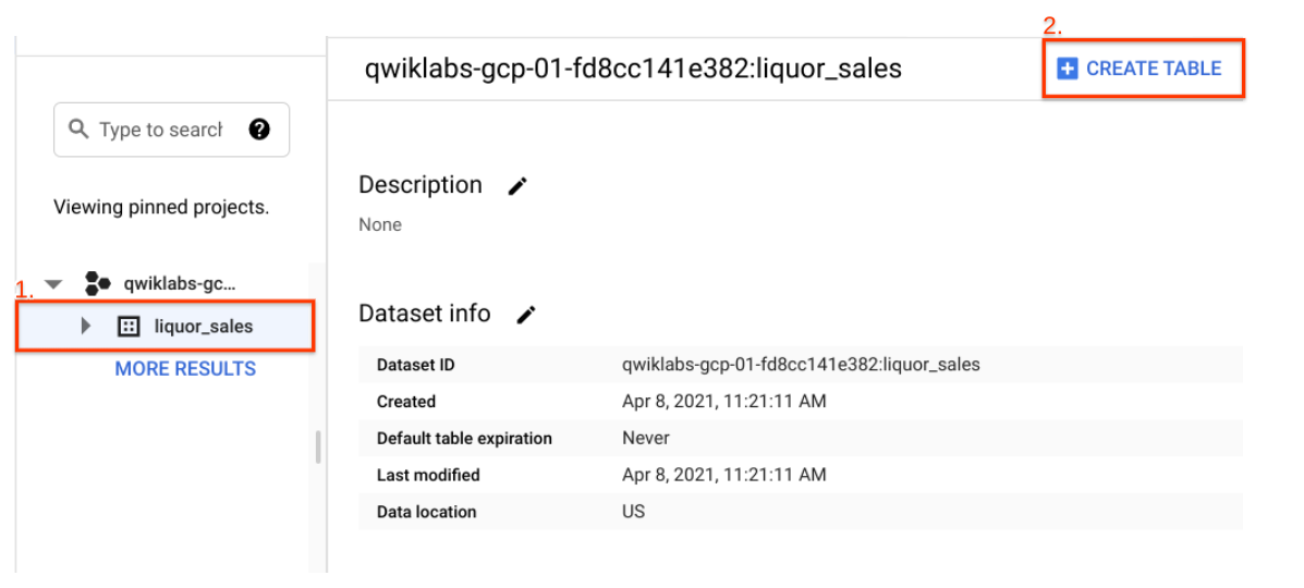
Task 1. Create a new dataset to store your tables

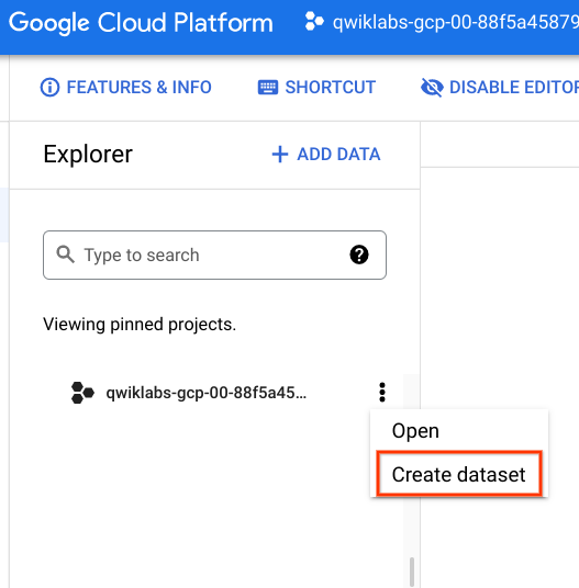
In your BigQuery project, create a new dataset titled liquor_sales.

1. In the Explorer section, click on the View actions icon next to your project ID and select Create dataset.

The Create dataset dialog opens.

2. Set the dataset ID to liquor_sales. Leave the other options at their default values, and click Create dataset.

In the left pane, you see a liquor_sales table listed under your project.

Task 2. Load and query relational data

In this section, you measure query performance for relational data in BigQuery.

BigQuery supports large JOINs, and JOIN performance is good. However, BigQuery is a columnar datastore, and maximum performance is achieved on denormalized datasets. Because BigQuery storage is inexpensive and scalable, it's a good practice to denormalize and pre-JOIN datasets into homogeneous tables. In other words, you exchange compute resources for storage resources (the latter being more performant and cost-effective).

In this section, you will be doing the following:

• Upload a set of tables from a relational schema (in 3rd normal form).
• Run queries against the relational tables.
• Note the performance of the queries to compare to the performance of the same queries against a table from a denormalized schema containing the same information.

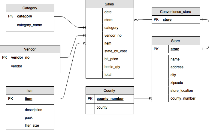
You upload tables that have a relational schema. The relational schema consists of the following tables:

Here's a diagram of the relational schema.

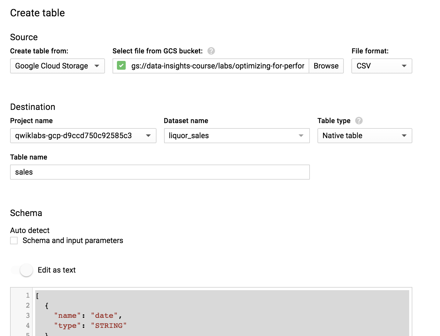
Create the sales table

1. In the Explorer section, click on the View actions icon next to the liquor_sales dataset, select Open, and then click Create Table.

2. On the Create Table page, in the Source section, do the following:

• For Create table from, choose Google Cloud Storage.
• Enter the path to the Google Cloud Storage bucket name:

• For File format, choose CSV.

3. In the Destination section, configure the following:

• For Table name, enter sales.
• Leave the remaining destination fields at their defaults.

4. In the Schema section, you configure the following:

• Click Edit as text.
• Copy and paste the below schema:

5. Click Advanced options to display and configure these options:

• For Field delimiter, verify that Comma is selected.
• Because sales.csv contains a single header row, set Header rows to skip, to 1.
• Check Quoted newlines.
• Accept the remaining default values and click Create Table.

BigQuery creates a load job to create the table and upload data into the table (this may take a few seconds).

6. Click Personal History to track job progress.

Create the remaining tables

Create the remaining tables in the relational schema using Cloud Shell command line.

1. Create the category table:

2. Create the convenience_store table:

3. Create the county table:

4. Create the item table:

5. Create the store table:

6. Create the vendor table:

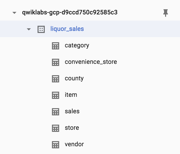
7. Go back to the BigQuery web UI. Confirm you see the new tables loaded into your liquor_sales dataset. Refresh the browser if needed.

Query relational data

Next, you use the Query editor to query your data.

1. Under the Query editor code box, click More > Query Settings.

2. In the Resource management, Cache preference section, uncheck the Use Cached Results checkbox and click Save. If you have to run the query more than once, you don't want to use cached results.

3. In the Query editor window, enter the following query against the relational tables and click Run:

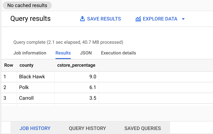
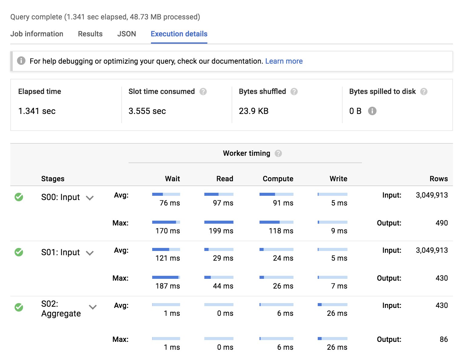
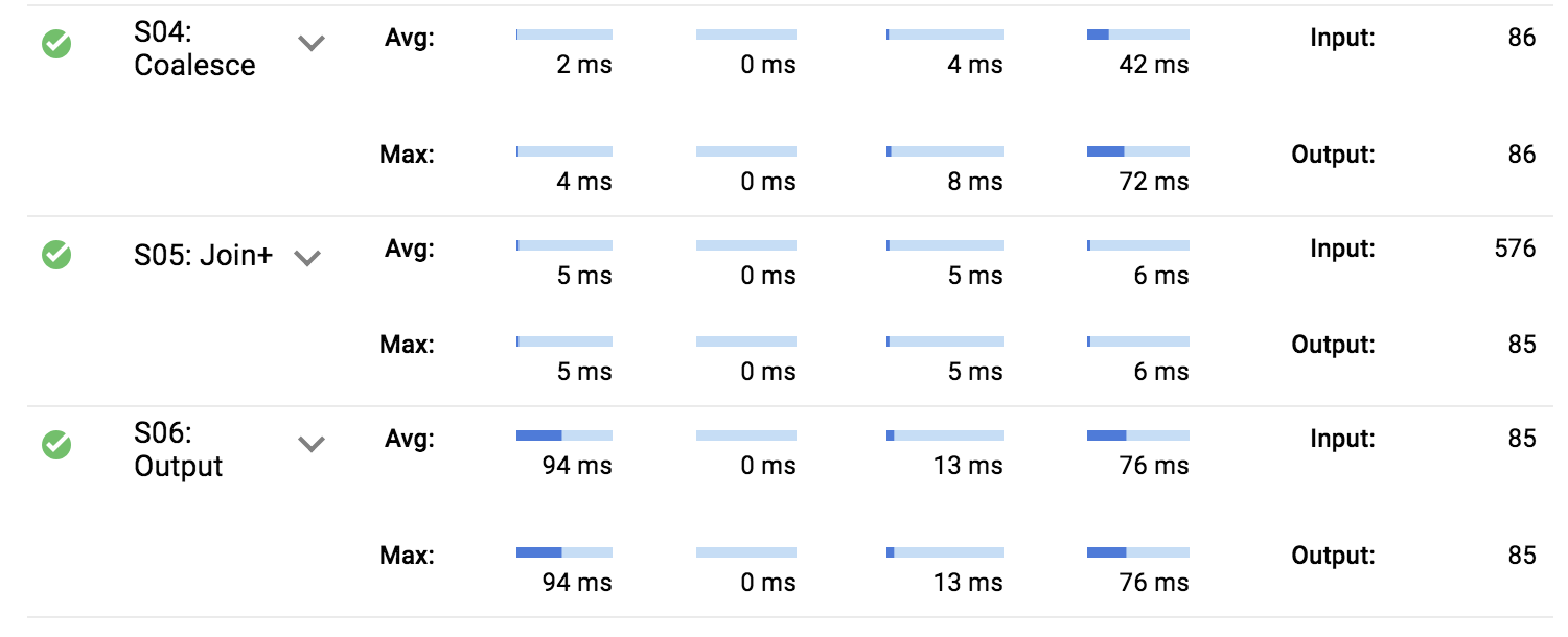
4. At the bottom, in the Query results section, click on the Results tab. Note the Query complete time. An example is shown below (your execution time may vary).

This will be compared to the time to query a flattened dataset in later sections.

Task 3. Load and query flattened data

In this section, you denormalize the schemas and analyze liquor sales for the state of Iowa using the flattened data. Running this query on the flattened data should be faster than running on the relational data. You will note the time to compare and confirm.

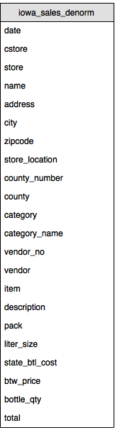
A denormalized schema flattens all relational data into a single row. For example, in the denormalized schema, county_number, county, store, name, address, city, zipcode, store_location, county_number, and cstore are fields containing all fields from the County, Store, and Convenience_store tables.

The following diagram shows the denormalized schema.

Create the iowa_sales_denorm table

1. In the left pane, select liquor_sales dataset and click Create Table on the right.

The Create table dialog opens.

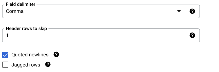
2. In the Source section, configure the following:

• For Create table from, choose Google Cloud Storage.
• Enter the path to the Google Cloud Storage bucket name:

• For File format, choose CSV.

3. In the Destination section, configure as follows:

• For Table name, enter iowa_sales_denorm.
• Leave the remaining destination fields at their defaults.

4. In the Schema section, configure the following:

• Click Edit as text.
• Copy and paste the below schema:

5. In the Advanced options section, configure as follows:

• For Field delimiter, verify that Comma is selected.
• Because iowa_sales_denorm.csv contains a single header row, for Header rows to skip, enter 1.
• Check Quoted newlines.
• Accept the remaining default values and click Create Table.

BigQuery creates a load job to create the table and upload data into the table (this may take a few seconds).

6. Click Personal History to track job progress.

7. Enter and run the following query against the table with a denormalized schema (this query produces the same results as the query in the previous section):

8. At the bottom, in the Query results section, click on the Results tab, note the Query complete time. This will be compared to the time to query a flattened dataset in later sections.

9. Note the time the query takes to run by subtracting the Start Time from the End Time.

Notice that the query corresponding to the table with denormalized schema runs slightly faster, and has simpler syntax. Wherever possible, pre-JOIN datasets into homogeneous tables to optimize performance in BigQuery.

Compare query performance with execution details

1. Select PROJECT HISTORY.

2. Click the first query job you ran against the normalized relational schema, then click OPEN AS NEW QUERY.

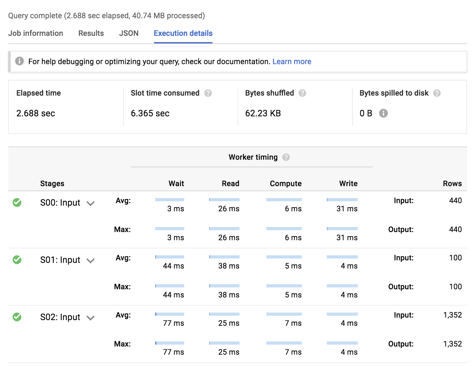
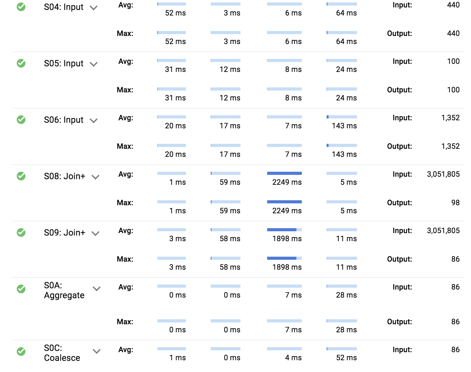
3. Select Execution details.

The execution plan has two major sections:

• Average and max worker timing by type of work per stage

• High level perforomance benchmarks

  • Elapsed time: Total time for the query to process.
  • Slot time consumed: If the query were not processed in parallel on multiple machines, how long would it take to process.
  • Bytes shuffled: Automatic in-memory data shuffling for massive parallel processing.
  • Bytes spilled to disk: If data cannot be processed in memory, how much was spilled to persistent disk (usually data skew is to blame).

1. First, compare the benchmark timings between each of the queries we ran.

2. Next, compare the type of work where the workers spent the most time.

Query 1. Relational schema execution details

Query 2. Denormalized schema execution details

Observations:

• The denormalized query (#2) is faster and uses less slot time to achieve the same result.
• The relational query (#1) has many more input stages and spends the most worker time in joining the datasets together.
• The denormalized query (#2) spends the most time reading data input and outputting the results. There is minimal time spent in aggregations and joins.
• Neither query resulted in bytes spilled to disk which suggests out datasets are likely not skewed (or significantly large enough to spill out from memory from an individual worker).

Avoiding performance anti-patterns

Now that you are familiar with effective database schema design, it is time to practice optimizing some poorly written queries.

The below query is running slowly, what can you do to correct it?

1. Copy and paste the below query into the Query editor and run the query to get a benchmark.

Goal: Count all the U.S. non-profit organizations that have filed taxes using paper (non-electronic) in 2015.

What can you do to improve the performance?

2. Compare against the below solution:

3. Run your updated version and track the time.

4. Clear the Query editor.

This new below query is running slowly. (Run the query to get a benchmark; stop after 30 seconds if it does not complete).

Goal: Using the Employer Identification Number (ein) as a linking field, join together the tax return filings table with the organizational names table and return the names of all the organizations that filed in 2015.

5. Add this query in the Query editor, then click Run:

6. Correct the above query. (Hint: Remember the correct JOIN field condition for our schema).

Compare against the below solution.

7. Add this query in the Query editor, then click Run:

8. Run your updated version and track the time.

Do you see an improvement? How quickly does the query run?

Lessons learned

Congratulations!

This concludes this hands-on lab looking at Effective BigQuery Schema Design and Query Performance. You have loaded CVS and JSON files into BigQuery tables, transformed data and join tables, stored query results, and then confirmed that data was transformed and loaded correctly.

End your lab

When you have completed your lab, click End Lab. Google Cloud Skills Boost removes the resources you’ve used and cleans the account for you.

You will be given an opportunity to rate the lab experience. Select the applicable number of stars, type a comment, and then click Submit.

The number of stars indicates the following:

• 1 star = Very dissatisfied
• 2 stars = Dissatisfied
• 3 stars = Neutral
• 4 stars = Satisfied
• 5 stars = Very satisfied

You can close the dialog box if you don't want to provide feedback.

For feedback, suggestions, or corrections, please use the Support tab.

Copyright 2022 Google LLC All rights reserved. Google and the Google logo are trademarks of Google LLC. All other company and product names may be trademarks of the respective companies with which they are associated.